Tagnetwork

2017 Spring AI Project – PoNNg

Towards the end of my first year at Virginia Tech, I oddly found myself with more free time than usual. Throughout the year I tried to focus on my neural network study when I could, but sadly, little time arose for me to pursue what I love. However, I always worked on small projects when I could. The majority of this time was spent geared towards learning Linux and Python, both of which I have become somewhat proficient in. Using these newfound skills, I looked back to my roots to see what improvements I could make on my original code from high school and to get back into the field of artificial intelligence in general. The main goal for this project was to create a short, dependable neural network algorithm for personal use in Python. I also wanted to create a system in which 2 neural networks were pitted against each other in some form of competition. I thought pong was a suitable game for this purpose because of its simplicity and competitive nature. My version of it stays, for the most part, true to the original game. 2 paddles, 1 ball, reset and score increase upon the ball exiting the left or right screen. After each bounce, the ball’s y velocity is randomly chosen between [2, 5] to add some randomness to where the ball will be when it reaches the left or right side of the screen. Pygame was used to render the components onto a window.

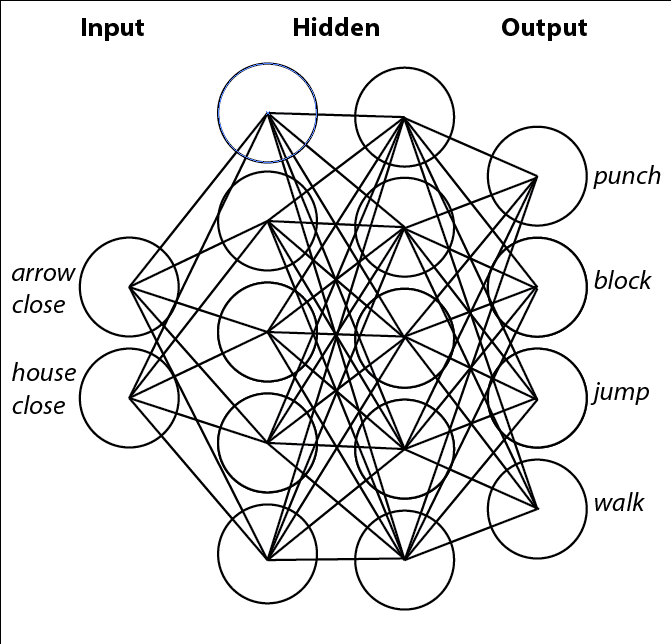
The general frame of mind I had while creating the neural network algorithm for this project was brevity and simplicity. One of the main issues with my Java implementation from a year ago was the fact that all of the weights were stored in a single 1D array, which isn’t ideal for many reasons. Mainly, it’s confusing to look at and understand the math behind extracting the correct weight at the correct time. To correct this, I switched it from a 1D array to a 3D array, in the format of [layer][input][output], layer being the current index in regards to the hidden layer, input being the “left” set, and output being the “right” set (i.e. input -> hidden, input is the “left” set and hidden is the “right” set). Although confusing at first due to my lack of experience with 3D arrays, I eventually came up with a good system that works just as fine as the original and is slightly easier to understand from an outsiders point of view. e

Screenshot from 2017-04-09 19-13-31

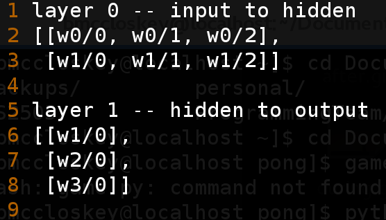
Example of a 3D weight storage system for a neural network with 2 input nodes, 1 hidden layer of 3 nodes, and 1 output node. The number of rows corresponds to the “input” layer (input -> hidden; input is the input layer, hidden -> output; hidden is the input layer) and the number of columns corresponds to the “output” layer (hidden and output in the above example).

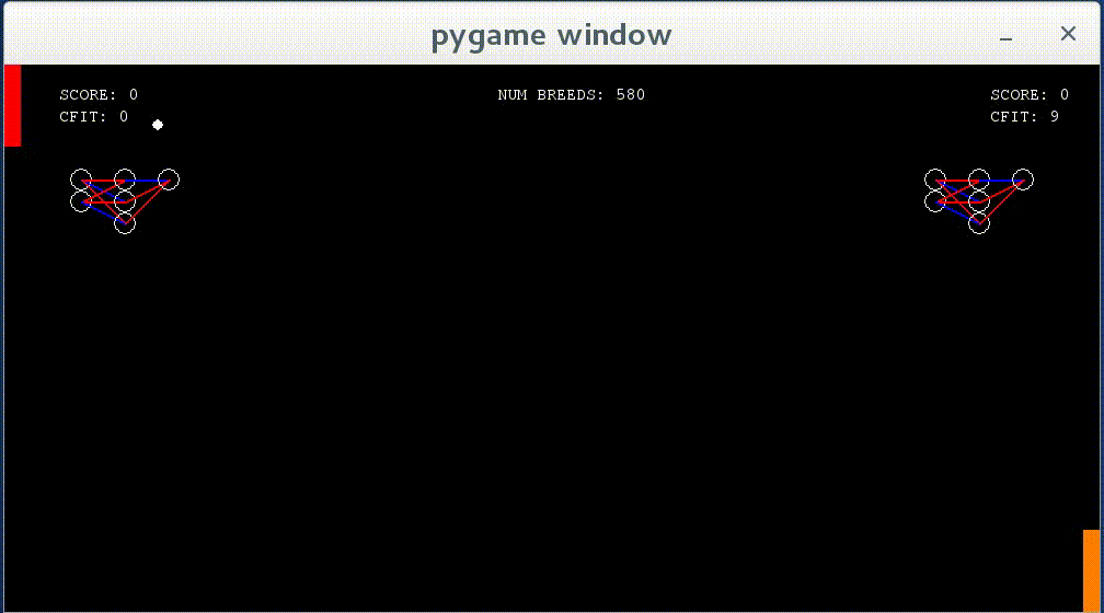
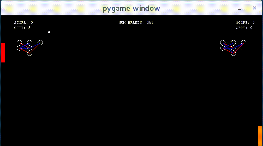
In this project, I experimented around with neural networks of varying sizes before settling on a simple 2 node input, 3 node hidden layer, and 1 node output network. The input was the vertical and horizontal distance between the paddle and the ball over the total height/width of the game window. When given more input nodes like the x and y velocity of the ball, it was observed that the neural networks were able to accurately predict where the ball would hit the paddle when it reached the side of the window (as opposed to just following the ball’s y component), but the time it took to reach this point was incredibly long and results varied over different situations (i.e. the angle the ball was approaching the paddle, etc.). Fitness was given based on how many matches the neural network won, but was punished twice as hard for every match (first to 3 points) lost (+1 for win, -2 for loss). A standard breeding process was performed after each match in which the parents were the 2 best performing networks in a population and the child was the worst, with the child weights having 2/3 chance of being from either of the parents and 1/3 chance of being the average of the parent weights. There was a 6% chance of any weight being erased and assigned a random value between (-1, 1). After each match, the loser was replaced by a randomly selected network from the population (it was ensured that the two networks playing each other were not the same one). Each paddle’s neural network can be seen displayed on its side of the board — each circle being a node and each line being a weight. A blue weight signifies a negative value and a red weight signifies a positive value.

Getting on to the actual project, the rate at which the neural networks became “good” at the game varied on each run. In my experience, it could be as short as 100 breeds, and as long as around 2000. However, for each run, the neural networks followed the same general pattern every time — make no attempt to move for the ball, show some attempt at chasing the ball or “reacting” the ball when it came close, and successfully chasing the ball.

before

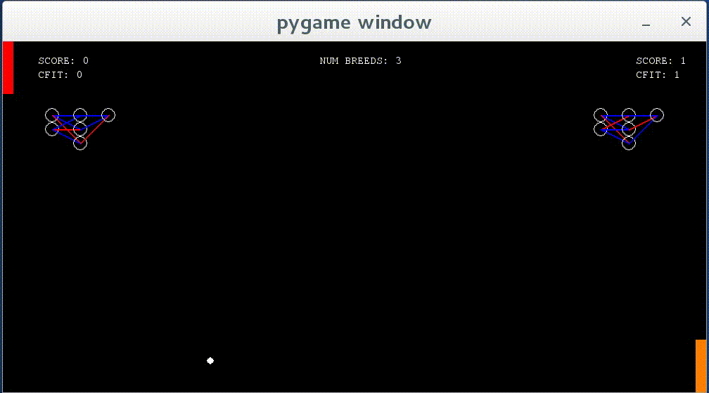
Right when the program started. You can see the paddles move to either the top or the bottom of the screen, paying no attention to the ball.

during.gif

Networks show some learning — they now react to the ball when it approaches them, though they do not move to the correct y value as of yet.

after

The end of the pattern. Networks demonstrate ability to chase after the ball and hit it every time. At this point, the match time is indefinite.

Although this project seemed simple at first, there were many different stages it went through while in development. At first, the input size for the neural networks was complex (including paddle location, ball location, ball velocity). However, after a lot of playing around, consistent improvement was shown when this list was refined to just the distance between the paddle and the ball. In retrospect, this makes sense, as decreasing the complexity of any problem makes it easier to solve. Although, maybe with more patience, a more unique strategy could have been developed with more inputs. I encourage you to download my source code and play around with yourself if you are at all interested in doing so (here).

2016 Spring AI Project – Floppo Bordo

As my senior year of high school began to slow down and the college hype began to increase, I looked for simple projects to work on while in the midst of the craziness. I spent a while sitting back and looking at the projects I’ve finished this past school year and remembered a couple of other projects from other people that served as inspiration for my personal projects. Since I learned everything I know about AI from watching lectures and demonstrations online, it was a trip down memory lane to go back and watch those videos in particular. One of the projects I looked back at was a machine learning algorithm that used reinforcement learning for Flappy Bird (A popular mobile game), and I remember being amazed at the actual process of learning that the algorithm went through (see that video here). I decided to challenge myself by making my own Flappy Bird AI to benchmark my current progress, especially in comparison to where I was 6 months ago.

First, however, I had to make a Flappy Bird clone. Making it was surprisingly easy, as it has simple rules and doesn’t require a lot of complex algorithms. Flappy Bird is essentially an endless runner, but the player must tap the bird to fly precariously in between pipes (if the player touches one of these pipes they die and have to start over). Since this was just a quick project, I didn’t bother with making images to go over each of the objects, instead using colored rectangles. The blue rectangle is the player, the black rectangles are pipes, and the green rectangle is the ground.

I used my standard Neural Network algorithm with a genetic algorithm for the machine learning AI (read more about Neural Networks here). It uses 4 inputs – the player’s y position (height from the ground), the y positions of the opening between the closest pipes (the lowest point on the top pipe and the highest point on the bottom pipe), and the horizontal distance between the player and the closest pipe. There are 2 hidden layers of 5 nodes each, and 1 output node (if the output node > 0.5, the bird jumps). I used a sigmoid function (1 / (1 + e^-x)) as my activation function. Reward was based on the score at the end of the run and how far the AI moved the bird to the right.

Now onto the results. It actually learned to jump between pipes fairly quickly, but difficulty came when it needed to jump with precision between the pipes. However, after a little bit of time, it mastered the game perfectly.

start

Start of the simulation. You can see the AI has trouble handling its own jump height.

stend

After about 10/15 minutes of runtime, the AI has mastered the art of jumping in between the pipes.

I enjoyed making this project and seeing how far I’ve come. A while ago, I never would have thought I would have been able to make something like this. If you want to see the code for this project, you can get it here.

2016 Spring AI Project – LD33 & Neural Networks

As my senior year of high school began to slow down and the college hype began to increase, I looked for simple projects to work on while in the midst of the craziness. Thinking that it had been a while since I had made anything relating to artificial intelligence, I wanted to refresh my mind on Neural Networks and machine learning in general. Since I needed a game to attach an AI to, I naturally thought back to my Ludum Dare 33 game (linked here), as it was a rather simple game that wouldn’t be hard for a computer to master.

I used a Neural Network (read more about Neural Networks here) with 2 input nodes (one to tell when an arrow was close and another to tell when a house was close), 2 hidden layers of 5 nodes each, and 4 output nodes (controlled each of the 4 keys required to play the game: punch, block, jump, move right). The activation function was again a sigmoid (1 / (1 + e^-4.9x)). I used a genetic algorithm with a 10% mutation rate on each gene passed down in order to weed out bad Networks and incentivize growth of good Networks.

Screen Shot 2016-03-25 at 11.11.00 PM

Graphic displaying the structure of the Neural Network I used for this project. Inputs were either a -1 or a +1 depending on whether or not its specific object was close (-1 for false, +1 for true). A key was pressed if its respective output value was > 0.5 (the range for the sinusoid I used was (-1, 1)).

Despite my belief that my game was easy, initial runs of the simulation proved that although scoring points was easy, there were too many ways to earn points, which confused the networks. The Networks easily figured out that moving right was a good way to earn points as points were given based on how many civilians are squished, but it had a hard time figuring out that it could squish civilians longer if it blocked arrows. However, after many many iterations, Networks could generally figure out a better strategy for scoring (whether it be jumping on houses to destroy them or blocking arrows). Despite the Networks learning how to score points better, I have yet to see a perfect strategy formed (one that jumps on houses AND blocks arrows), which may be solved if I ran more iterations of the simulation.

ld33aistart.gif

Starting out you can see that it doesn’t do anything. Usually, if it does anything, it holds down random keys, causing its actions to be sporadic at best.

ezgif-2212419532.gif

After ~5 minutes of the simulation running, the AI finds out that walking right is a good strategy for getting points.

ld33aiBLOCK.gif

After a considerably long time, the AI has figured out blocking is a good combo with walking, as it can walk longer distances than if it wasn’t blocking. However, it hasn’t found out that destroying houses is a good source of points.

All in all I think this was a great refresher for AI. Since I’ve been mostly working on games these past few months, it was also a good break from the grind that asset creation is becoming. Also, learning that machines aren’t always as bright as I may think they are is a great lesson to take going forward in my AI career. If you want to see the code for this you can see it here: https://github.com/mccloskeybr/LD33

© 2024 Brendan McCloskey

Theme by Anders NorénUp ↑