2017 – Brendan McCloskey

Tag2017

2017 Fall Cluster Project – Raspberry Pi 3 Cluster

After using VT’s cluster for so long, I was interested to learn how the computing behind it worked, and decided to make my own cluster of Raspberry Pis. I contemplated the benefits of embarking on such a project and came up with a multitude of experiments I was interested in exploring that would benefit a cluster-like structure, of which include password decryption, simulation for genetic algorithms, and more. What really tipped me over, however, was the already written and free to use libraries MPI and MPI4PY, of which allowed me to use python to write easy to understand and easy to implement code that utilized cluster computing. Thankfully I had a lot of the components on hand already, but I estimate the overall cost to be around $270. This includes the cost of 4 Raspberry Pis, 4 8gb micro SD cards, a stand for the pis, an ethernet switch, 5 ethernet cords, a USB hub, and 4 micro USB – USB cords. There’s a great video series by Tinkernut on Youtube that I used for basic reference when configuring my Pis that I’d certainly recommend you follow along as well if you have any difficulties putting one of these together. If you have any questions about any of the components I used to build my cluster, feel free to email me at [email protected].

For my cluster, I used 4 Raspberry Pi 3 B boards, each running a distribution of CentOS 7 Linux. I decided to use CentOS 7 over a friendlier version of linux (i.e. Raspbian, a distribution written specifically for the Pi), simply because VT’s cluster also uses CentOS. Each Pi is given power and connected to an Ethernet switch that is also connected to my router so I can ssh into each of the nodes.

Picture of my cluster

I have the Pis set up in a master-slave system, in which the head node takes one big problem and divides it into smaller problems for the slave nodes to compute. This allows me to, say, run genetic algorithm/ANN simulations on the slave nodes while performing breeding and fitness evaluation on the master node. I definitely plan on experimenting with speedups in regards to AI in the future, so be on the lookout.

After building my cluster, I found it fitting to at least write a short piece of test code to see how much the cluster structure sped things up. I decided to time Leibniz’s Pi approximation to the 100,000th term on a single worker vs. all three workers. You can see the results of that experiment below.

Screen Shot 2017-11-22 at 9.04.51 PM
Testing 1 vs. 3 workers

You can see that the test in which I only used one worker (nodelist_small), the runtime was approximately 3 times as large as the runtime when I used 3 workers (nodelist), which is to be expected. You can also see that the estimates are slightly different, though I believe this error to be a result of integer division losing some information when divvying up the work for slave nodes (As this is just a small test, I’m leaving this error for now). You can get the code for this test here.

This was an incredibly fun and practical project to work on during my Thanksgiving break. Definitely be looking for more updates from me as I begin to experiment more with the cluster and what it can do. Hopefully I can run some experiments before my next break, but as exam season is coming up, I may need to focus more on my studies. If you have any questions or comments, feel free to email me or leave a comment.

When idle, my cluster is aiding the BOINC sponsored SETI@Home project. I chose this over other BOINC projects mainly due to it’s friendliness towards ARM processors (of which the Raspberry Pi uses).

2017 Fall Data Analytics Competition – VT/GDMS Health in the US

November 7, 2017 / mccloskeybr / 1 Comment

Moving into the fall semester of my Sophomore year at Virginia Tech, I was a little starved of side projects I could do, simply due to the amount of schoolwork I had to finish each week. However, luckily I was able to make time for a couple projects I could focus on in the side. One of them being is data analytics competition, of which was sponsored by the CMDA club here at VT and GDMS. I participated in the beginners competition in a group of 3, the other members being good friends of mine Eric Fu and Kali Liang. In the competition, we were given a large data set (.csv file) involving health issues across various cities throughout the United States (500 entries). Some examples of the categories, just to get a feel of the type of data we received, included ailments such as asthma, obesity, heart disease, kidney disease, etc. We were also given general data involving disease prevention (i.e. access to health care, going to regular checkups, etc.) and unhealthy behaviors (i.e. binge drinking, drug use, lack of leisure time and sleep, etc.).

I believe that my group’s approach to the data was a rather unique one, given our different backgrounds. Eric is a BIT major, Kali is a CMDA (Computational Modeling and Data Analytics) and Statistics major, and I am, of course, a Computer Science major. As a result of our different backgrounds, we each had different ideas as to how to approach the information to find correlations between the categories. For instance, my approach was to code basic programs in Python using numpy and matplotlib to generate scatterplots and other useful graphs, while Kali was comfortable using R to find more statistics-heavy information (like GLM/LS Means) and Eric was comfortable working directly in the given Excel file to look for correlations.

First, we decided as a group to look for interesting differences in the data by splitting the it up into regions. We explored a number of splits, and we ended up using data from a regional split (NE, S, MW, W), a coastal split (west/east coast, with everything else being lumped into a “main land” group), and a split based on population size to explore the uniqueness of big cities (we defined a big city as any city above 2 standard deviations above the mean population for the entire data set). We also explored a split based on State, but found the data to be too volatile, and with 51 groups (incl. Washington DC), there were still too many points to investigate. My python scripts came into good use here, as I was able to make a quick program that found and graphed the scatterplots of each region for any given category, along with a line that connected the means for each sub group together (with and without outliers) for visual investigation. I also coded a script that plotted scatter plots for any 2 given categories to see if they were related.

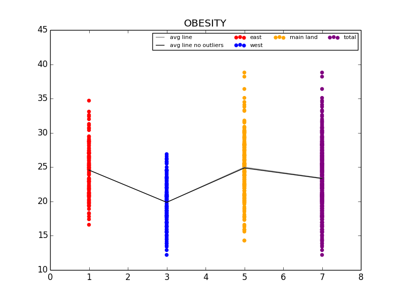
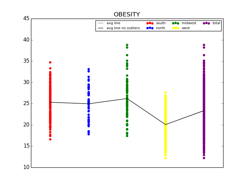
The first graph details the difference in Obesity in the east vs. west coast, while the second illustrates the difference in Obesity in the US Regions.

From this initial stab at the data, we found what we believed to be significant differences between the general health in the east coast and the west coast (meaning the west coast was significantly lower than the east in almost all categories). Also worth noting, we also determined that health in the west region was generally better than the other regions. From this lead, we explored the differences in the means to attempt to understand why the west is generally healthier. We observed that both the west coast and the west region have significantly lower Obesity rates when compared to other regions, and decided to explore that as a possibility (see the mean comparison charts above). We confirmed our assumption by looking at the general trends for obesity and various other ailments and observed that, in general, there is a strong link between obesity and other serious health problems.

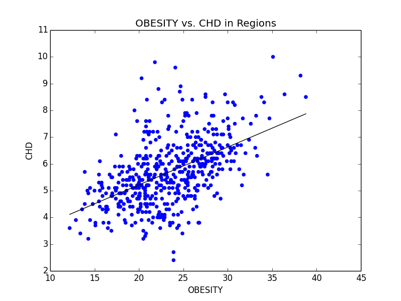
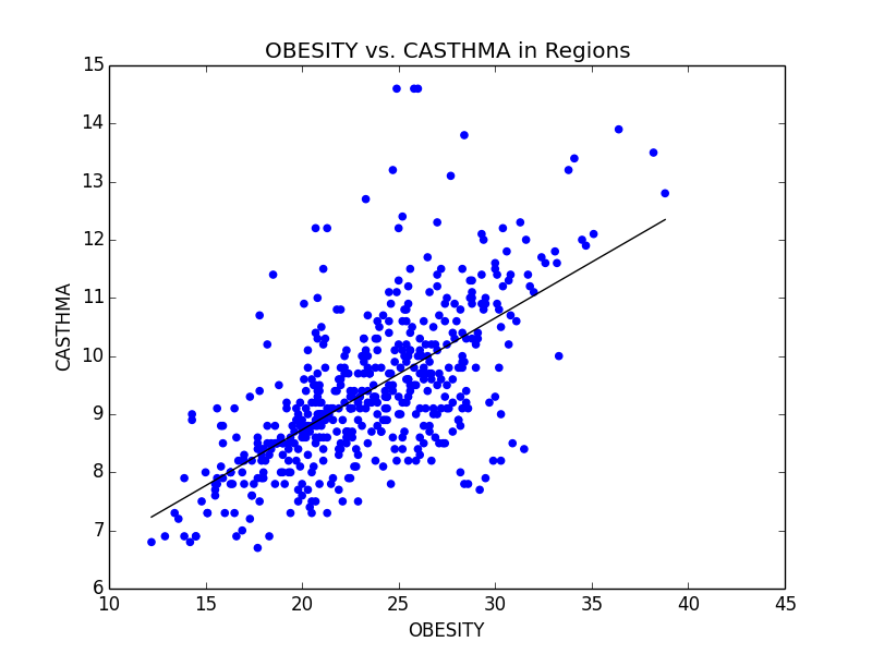
Some of the scatterplots we used to illustrate the link between Obesity and other serious illnesses like heart disease (CHD) and asthma (CASTHMA).

In order to further provide evidence for our assumptions, Kali used regression analysis, specifically generalized linear models with least square means to further look for significance between these groups. Using these tests was helpful because it not only aided at eliminating some of the confounding variables that may be lurking within the data, but made it extremely clear as to whether the data was significant or not through looking at the p-value numerically and with a visual aide. Essentially, when graphed, intervals of the mean are plotted for each region (each interval determined using a 95% CI). If the regions don’t have any overlapping points, then the difference between the two can be considered significant and is definitely worth looking into. As you can see below, we were able to confirm our assumption that the difference between obesity rates in the east and west is significant.

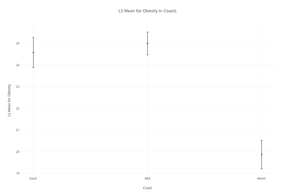
LSM Chart confirming our assumption that the difference in Obesity rates in the east and west coasts is significant

However, we were not satisfied simply stating that we recommend that Obesity rates be lowered, so we looked into possible variables that could affect Obesity that weren’t already included in our data set. Ideas for this included finding density of fast food restaurants within each city, and measuring the nutritional differences between each city. Unfortunately, we were unable to find any reliable data on density of fast food restaurants, but we were able to pull data from the CDC website pertaining to amount of people that ate less than one fruit and one vegetable per state in the US. Using this data, we first confirmed the link between not eating nutritional food and obesity, then went on to make our recommendation. Eric’s background in Business came in handy, as we gave various recommendations that made sense from an economics point of view (i.e. decrease the tax or cost of fruits and vegetables in obese regions, subsidize farmers to increase fruit and vegetable output, or push advertisements encouraging people to eat healthier).

As a slight aside to our main focus on Obesity across the US, we also found that Stress (we defined stress as a lack of leisure time (LPA) and a lack of sleep) was high in big cities. We noticed that not only were kidney problems slightly higher in bigger cities, but so were other ailments such as strokes and diabetes. We were able to link the connection between stress and diabetes with kidney problems (seen below), and further connect kidney problems with strokes. Unfortunately, due to the time constraints for the competition, we were not able to explore these connections much deeper. However, given more time, we definitely would have done so.

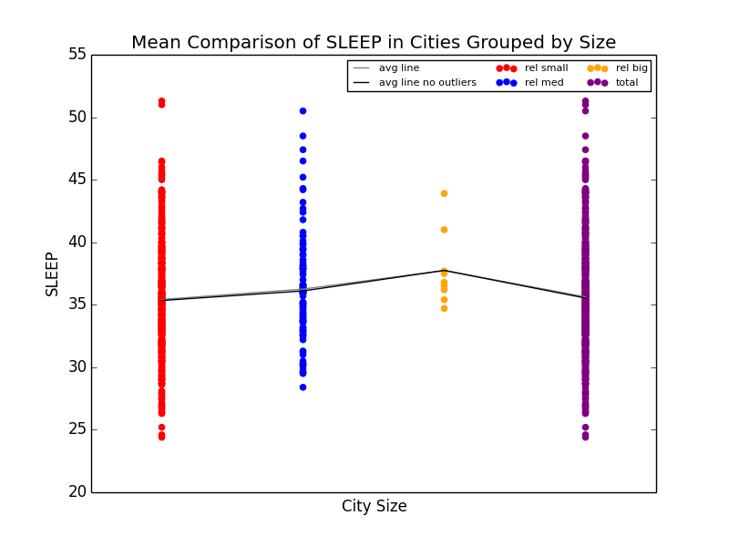
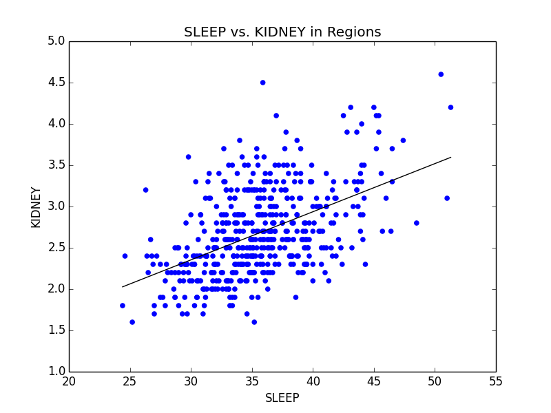
Mean comparison showing increase in lack of sleep in big cities and scatterplot showing the relationship between sleep deprivation and kidney problems.

This competition was extremely fun to participate in. Unfortunately, we did not place in the top 3 teams for our section, although we did get an honorable mention. I want to thank GDMS and the CMDA club at VT for making this a reality. I’ve always been interested in data analytics due to my background in neural networks, and it was incredibly fun to work on something data analytics related even though I haven’t been able to take any statistics courses as of yet.

If you’d like to see any more plots, or would like to see the scripts I made for the purpose of this competition, feel free to email me at [email protected].

2017 Summer App Project – The Stalk Market

August 15, 2017 / mccloskeybr / 0 Comments

As my previous post (linked here) eluded, this is the second and main project I worked on during the latter half of my summer break from Virginia Tech. Described shortly, this project is a stock market tracker of sorts for the game Animal Crossing: New Leaf (ACNL) that is able to run from any handheld Android phone. My main focus for this project was introducing myself to the world of app development, mainly following various tutorials online and playing around with the Android Studio IDE. As such, the actual logic behind this project isn’t too difficult to grasp. As I’ll get into, the stock market in ACNL is rather simple and follows a strict set of rules. Thus, I mainly focused on making the user interface as fluid as possible, to ensure ease of use and practicality while keeping the function of the app in mind.

What the app looks like when you open it for the first time. I put a decent amount of effort into ensuring the app looks somewhat decent and is easy to use. Note, all pictures shown here are screenshots taken on my Google Pixel.

First, onto the basics of the stock market in ACNL. Every Sunday, the player can buy Turnips from a particular NPC that visits the town. The price for that particular set of turnips can range anywhere from 90-110 bells (the currency of ACNL). Then, throughout the week, the selling price of those turnips changes depending on the particular pattern for that week. The prices change twice per day (at store-open and 12pm), with the turnips rotting at exactly 6am on Sunday. Thus, the player must guess when he or she should sell all of the turnips they purchased for that week to ensure maximum profits. This is where my app comes in. The user is to enter every price update in-game into the app. Then, when prices are optimal, the app recommends the user to sell all of their turnips.

There are 4 patterns the stalk market can have for any given week, each with its own set of rules that makes it easily distinguishable from the others. Of the patterns that produce positive returns, the player is first tempted multiple times with above average selling prices before the maximum price is observed. The biggest example of this is the big spike pattern, where there are 2 above average prices before the best price, often double that of the previous prices, is observed. My app guesses which pattern is most likely for the given week/set of values, and warns against selling your turnips until it thinks the highest value for the week has been achieved. There is only one pattern in which the player is guaranteed a loss. If you’d like to read more on the various patterns and their strategies, I would recommend visiting this page.

Though the turnip price in the first picture is much higher than the purchase price (labeled in blue), the app recommends waiting, which pays off with a week-high price 3 times that of the previously shown price, as shown in the second picture.

Once the logic was finished and patted down, I moved onto the user interface portion of the app. The only non-native library I used was GraphView for the plot of prices seen on the upper-half of the screen. The main challenge when coming up with the UI for this project was where to place the buttons and text box in relation to each other and the graph. I ended up with the current design, as I think it looks and feels simple and easy to use. One of the previous designs had all of the buttons underneath the graph in a 2×2 grid pattern, which failed due to the strangeness of fingers as a cursor. Sometimes, I found myself pressing the bottom right button when I meant to press the upper left button, among other similar problems. I’ve found that the current vertical design is a clear and easy solution that wasn’t difficult to implement. Other than button placement, I used in-game and fan art (the background, turnip, and animal figure) for decorating the app. If I were to publish this on the Play Store, I would first want to draw myself or enlist the help of a friend to redraw all of these assets to ensure I didn’t steal content from their creators. As such, you will not be able to find this on the Play Store as of yet. However, if you email me saying you want to put this app to use, feel free to and I will post an app that falls within these guidelines.

This project was fun to explore. I learned a whole lot about Android app development, and created something I can put to use in my future ACNL endeavors. If you’d like to look at the source code, you can see it here.

2017 Summer Cryptography Project – Caesar Ciphers and ASCII Tables

June 26, 2017 / mccloskeybr / 1 Comment

Admittedly, the time before my summer semester in Japan was ill-spent in regards to furthering my understanding in the Computer Science world. However, there were still a couple of projects that I did for fun before I left. This first project, a rather simple caesar cipher, was the first of two projects I did. I did this project in particular as a way to brush up on some of the knowledge of the C language I gained during my spring semester CS 2505 class at Virginia Tech. For those unfamiliar with the concept of a caesar cipher, it’s a crude way to encode a chunk of information — simply taking every letter and shifting it up or down a predetermined number of spaces in the alphabet. For instance, the string “abcd” would be encrypted to “bcde” with a caesar key of positive one. Of course, traditionally, wrapping occurs at the ends of the alphabet; meaning z -> a with a key of +1, and a -> z with a key of -1.

There are a couple key parts when it comes to translating this into code. First and foremost, I made it runnable via. the command line. The program expects the file path to the text file the user wants scrambled or unscrambled, along with either ‘e’ or ‘d’ for ‘encode’ and ‘decode’ respectively. Next, instead of letting the letters wrap once at the end/beginning of the alphabet, I allowed the characters to go above/below this limit, possible thanks to the format of the ASCII table.

asciifull

ASCII table

In C, along with the vast majority of programming languages used today, ‘char’ (character) variables are actually stored as integers. Each character is 1 byte, allowing for up to 256 different characters to exist. This not only includes your standard upper/lower case alphabet and numbers, but also special characters, along with some special, machine only characters, like ‘\n’ (new line). So, instead of wrapping at the ends of the alphabet, I wrapped at the ends of the ASCII table (see methods encode and decode in the block below to see how). In regards to my program, this is relevant because it allows for characters to spill over into generally weird or unexpected characters, making it easier on us to program because we don’t need to look for specific ASCII values to wrap around, as well as adding a bit more effectiveness to the final product. Of course, this method won’t fool someone who knows what they’re doing when it comes to decryption, but it should generally prevent friends or co-workers from snooping into information you don’t want shared.

There are still plenty of improvements that can be made to this system to improve it even further and lessen the chance of someone cracking a particular files key. As you can see in this iteration of the program below, the key is static between all files, meaning a correct guess on one file means access to your entire library of secret text files. This could be improved by simply making the key random between files and stored somewhere inconspicuous. For instance, the key could be between 0 and 255, and simply written as the first character of the encoded file. While again, this method would fail almost instantly in the case of a professional crack, it should stump the average Joe for a couple of hours. Or, perhaps this method is repeated for every character in any one file; the key for any given character placed just before or after it. I’m sure you can see how this method can become increasingly complex, and increasingly difficult to break, the longer you think about it.

FILE *f;

int caesar = 5;

int main(int argc, char **argv) {
	if (argc != 3)
		badInput();
	FILE* f = getFile(argv[1]);
	if (strcmp(argv[2], "e") == 0)
		encode(f);
	else if (strcmp(argv[2], "d") == 0)
		decode(f);
	else
		badInput();
	fclose(f);
	return 0;
}

void badInput() {
	printf("Format is '.../caeser <.../fileToEdit.txt> <e/d>'\n");
	exit(1);
}

FILE* getFile(char *url) {
	FILE *f = fopen(url, "r+");
	if (f == NULL) {
		printf("Can't locate file '%s'", url);
		badInput();
	}
	return f;
}

void encode(FILE *f) {
	int c;
	while((c = fgetc(f)) != EOF) {
		fseek(f, -1, SEEK_CUR);
		fputc((c + caesar) % 255, f);
		fseek(f, 0, SEEK_CUR);
	}
}

void decode(FILE *f) {
	int c;
	while((c = fgetc(f)) != EOF) {
		fseek(f, -1, SEEK_CUR);
		fputc((c - caesar) % 255, f);
		fseek(f, 0, SEEK_CUR);
	}
}

The C code behind the Caesar Cipher. If you have any questions about the code feel free to email me: [email protected].

This project was an easy, quick, and fun way to stay familiar with the ins and outs of ASCII values and C I/O alike. Feel free to take this idea further and create ciphers of your own!

2017 Spring AI Project – PoNNg

April 10, 2017 / mccloskeybr / 2 Comments

Towards the end of my first year at Virginia Tech, I oddly found myself with more free time than usual. Throughout the year I tried to focus on my neural network study when I could, but sadly, little time arose for me to pursue what I love. However, I always worked on small projects when I could. The majority of this time was spent geared towards learning Linux and Python, both of which I have become somewhat proficient in. Using these newfound skills, I looked back to my roots to see what improvements I could make on my original code from high school and to get back into the field of artificial intelligence in general. The main goal for this project was to create a short, dependable neural network algorithm for personal use in Python. I also wanted to create a system in which 2 neural networks were pitted against each other in some form of competition. I thought pong was a suitable game for this purpose because of its simplicity and competitive nature. My version of it stays, for the most part, true to the original game. 2 paddles, 1 ball, reset and score increase upon the ball exiting the left or right screen. After each bounce, the ball’s y velocity is randomly chosen between [2, 5] to add some randomness to where the ball will be when it reaches the left or right side of the screen. Pygame was used to render the components onto a window.

The general frame of mind I had while creating the neural network algorithm for this project was brevity and simplicity. One of the main issues with my Java implementation from a year ago was the fact that all of the weights were stored in a single 1D array, which isn’t ideal for many reasons. Mainly, it’s confusing to look at and understand the math behind extracting the correct weight at the correct time. To correct this, I switched it from a 1D array to a 3D array, in the format of [layer][input][output], layer being the current index in regards to the hidden layer, input being the “left” set, and output being the “right” set (i.e. input -> hidden, input is the “left” set and hidden is the “right” set). Although confusing at first due to my lack of experience with 3D arrays, I eventually came up with a good system that works just as fine as the original and is slightly easier to understand from an outsiders point of view. e

Screenshot from 2017-04-09 19-13-31

Example of a 3D weight storage system for a neural network with 2 input nodes, 1 hidden layer of 3 nodes, and 1 output node. The number of rows corresponds to the “input” layer (input -> hidden; input is the input layer, hidden -> output; hidden is the input layer) and the number of columns corresponds to the “output” layer (hidden and output in the above example).

In this project, I experimented around with neural networks of varying sizes before settling on a simple 2 node input, 3 node hidden layer, and 1 node output network. The input was the vertical and horizontal distance between the paddle and the ball over the total height/width of the game window. When given more input nodes like the x and y velocity of the ball, it was observed that the neural networks were able to accurately predict where the ball would hit the paddle when it reached the side of the window (as opposed to just following the ball’s y component), but the time it took to reach this point was incredibly long and results varied over different situations (i.e. the angle the ball was approaching the paddle, etc.). Fitness was given based on how many matches the neural network won, but was punished twice as hard for every match (first to 3 points) lost (+1 for win, -2 for loss). A standard breeding process was performed after each match in which the parents were the 2 best performing networks in a population and the child was the worst, with the child weights having 2/3 chance of being from either of the parents and 1/3 chance of being the average of the parent weights. There was a 6% chance of any weight being erased and assigned a random value between (-1, 1). After each match, the loser was replaced by a randomly selected network from the population (it was ensured that the two networks playing each other were not the same one). Each paddle’s neural network can be seen displayed on its side of the board — each circle being a node and each line being a weight. A blue weight signifies a negative value and a red weight signifies a positive value.

Getting on to the actual project, the rate at which the neural networks became “good” at the game varied on each run. In my experience, it could be as short as 100 breeds, and as long as around 2000. However, for each run, the neural networks followed the same general pattern every time — make no attempt to move for the ball, show some attempt at chasing the ball or “reacting” the ball when it came close, and successfully chasing the ball.

before

Right when the program started. You can see the paddles move to either the top or the bottom of the screen, paying no attention to the ball.

Networks show some learning — they now react to the ball when it approaches them, though they do not move to the correct y value as of yet.

after

The end of the pattern. Networks demonstrate ability to chase after the ball and hit it every time. At this point, the match time is indefinite.

Although this project seemed simple at first, there were many different stages it went through while in development. At first, the input size for the neural networks was complex (including paddle location, ball location, ball velocity). However, after a lot of playing around, consistent improvement was shown when this list was refined to just the distance between the paddle and the ball. In retrospect, this makes sense, as decreasing the complexity of any problem makes it easier to solve. Although, maybe with more patience, a more unique strategy could have been developed with more inputs. I encourage you to download my source code and play around with yourself if you are at all interested in doing so (here).

Theme by Anders Norén — Up ↑

Brendan McCloskey

software developer

Recent Posts

Recent Comments

Archives

Categories

Meta